Figure 1: Empirical CDF and Power Law Fit in Firm Size
Distribution based on Revenue
Using Power Laws to Identify the Structural Parameters
of Trade Models with Firm Heterogeneity
Saad Ahmad
Zeynep Akgul
ECONOMICS WORKING PAPER SERIES
Working Paper 2017–05–F
U.S. INTERNATIONAL TRADE COMMISSION
500 E Street SW
Washington, DC 20436
May 2017
Special thanks to David Riker for valuable comments and suggestions.
Office of Economics working papers are the result of ongoing professional research of
USITC Staff and are solely meant to represent the opinions and professional research of
individual authors. These papers are not meant to represent in any way the views of the
U.S. International Trade Commission or any of its individual Commissioners. Working
papers are circulated to promote the active exchange of ideas between USITC
Staff and recognized experts outside the USITC and to promote professional
development of Office Staff by encouraging outside professional critique of staff
research.
Using Power Laws to Identify the Structural Parameters of Trade Models with
Firm Heterogeneity
Saad Ahmad and Zeynep Akgul
Office of Economics Working Paper 2017–05–F
May 2017
Abstract
While various firm heterogeneity models of trade have recently emerged in the CGE literature, their mainstream adoption in trade policy analysis has been limited partly due to lack of available parameter estimates at the disaggregated sector level. In particular, the productivity dispersion and substitution elasticity parameters need to be estimated in a manner consistent with the theoretical underpinnings of the firm heterogeneity framework. In this paper we address this gap by estimating the productivity dispersion parameter by using ORBIS firm-level data and imputing substitution elasticities by fitting the firm size distribution and productivity distribution to the Pareto distribution.
Saad Ahmad
Office of Economics, Research Division
saad.ahmad@usitc.gov
Zeynep Akgul
Center for Global Trade Analysis, Purdue University
Office of Economics, Research Division
zakgul@purdue.edu
Since the seminal work of Melitz (2003), a growing trend in trade policy analysis is to incorporate observed firm characteristics such as heterogeneity in productivity and size in the underlying theoretical framework. A reasonable argument can actually be made that the absence of heterogeneous firms in trade dynamics leads to an incomplete picture of overall welfare from changes in the trade environment. As a consequence, several firm heterogeneity models of trade in the Computable General Equilibrium (CGE) framework have emerged in recent years with the ability to explain trade and welfare effects of economic integration in greater precision (Zhai, 2008; Balistreri et al., 2011; Balistreri and Rutherford, 2013; Dixon et al., 2016; Akgul et al., 2016). As a result, this growing literature on firm heterogeneity is generating new economic insights for policy analysis.
As is the case with traditional trade models, chosen parameter values play a critical role in determining the welfare predictions from firm heterogeneity models. Thus, establishing the appropriate parameter values for use in these models is critical for accurate policy analysis. While there are a number of methodologies prevalent in the current literature for obtaining these parameters, they often lack consistency with the underlying firm heterogeneity theory, indicating a clear need for continued efforts towards theory-consistent parameterization of firm heterogeneity models (Akgul et al., 2015). Indeed, the lack of a general and theoretically-sound approach for obtaining parameters in firm heterogeneity models remain one of the main challenges in advancing their widespread adoption for policy analysis.
One of the reasons why identification of the structural parameters in the firm heterogeneity model is such a challenge is that there are more parameters to consider in the Melitz (2003) framework than in the traditional Armington trade models. The key parameter in Armington models is the trade elasticity term (Armington elasticity), which is generally estimated using gravity models.1 On the other hand, firm heterogeneity models have two structural parameters: the shape parameter of Pareto distribution for firms’ productivity () along with the elasticity of substitution across varieties (). Quantitative results of trade cost reductions on trade flows and welfare are sensitive to these structural parameters. The importance of the value of on trade patterns and welfare is quite established (Hertel et al., 2007; Kancs, 2010; Hillberry and Hummels, 2013; Feenstra, 2014). The value of is equally important in Melitz models. For example, di Giovanni and Levchenko (2013) show that in the case when the firm size distribution is fat-tailed (small shape parameter), the incumbent firms in the industry are large and have a disproportionate share of overall sales compared to the small marginal firms and the welfare impact of trade is driven by incumbent firms rather than the marginal ones. Therefore, the contribution of the extensive margin to trade is found to be negligible when the shape parameter is small. Moreover, in order for the Melitz model to be well-defined and the firm size distribution to have a finite mean, parameter values need to satisfy the constraint, , adding another layer of restriction in choosing appropriate parameter values.
To simplify some of the complexities, the majority of the Melitz implementations (CGE and non-CGE) adopt a set of trade elasticities from the existing literature (Balistreri et al., 2011; Eaton et al., 2011; di Giovanni and Levchenko, 2013; Melitz and Redding, 2013). There have also been some attempts to estimate these parameters directly from a structural model. For example, Crozet and Koenig (2010) rely on gravity equations and use French firm-level data to estimate the structural parameters in Chaney (2008), which are the shape parameter of productivity distribution, elasticity of substitution, and the distance elasticity of trade costs. They estimate three equations to identify the three parameters. Their first equation is a gravity equation that determines the intensive margin of trade by estimating firm export values. This estimation yields a combination of substitution elasticity and distance elasticity of trade costs. The second equation is another gravity equation that determines the extensive margin of trade, where the probability of firm export participation in a bilateral trade link is estimated. This yields a combination of the shape parameter and distance elasticity. The last equation is a rank-size distribution of productivity, where the firm-level TFP is estimated based on Olley and Pakes (1996). Finally, this estimation yields a combination of the shape parameter and substitution elasticity. They identify each parameter by solving the coefficient estimates in three equations. The resulting structural parameter values show considerable variation across the manufacturing sectors in their database.
Following the methodology in Crozet and Koenig (2010), Akgul et al. (2015) estimate a combination of firm heterogeneity parameters for manufacturings sectors using a two-stage estimation method with country and industry level data. Since aggregate data bases do not allow for individual identification of parameters, Akgul et al. (2015) rely on the shape parameter estimates of Spearot (2016) to impute the values of elasticity of substitution. While they provide significant improvement on the existing methods to obtain elasticity values that can be used in CGE models that incorporate Melitz (2003), they rely on other studies for the shape parameter. We extend their idea to provide parameter values that are consistent with the data base used, eliminating the reliance on outside sources for the shape parameter that may not be fully consistent with the Melitz (2003) framework.2
In this paper, we propose a simpler method to estimate the structural parameters of firm heterogeneity models that relies on the theoretical relationship between the size distributions of firms and the and parameters. The Pareto assumption for firm sales is equivalent to assuming that firm productivity is Pareto-distributed, though with a different shape parameter. In general, when firm productivity is from a Pareto distribution with shape parameter , then the firm size also follows a Pareto distribution, however, with a different shape parameter, , which in fact is a ratio based on the two structural parameters: (di Giovanni and Levchenko, 2013). Since can be estimated directly from firm-level data, it provides a useful way to infer the ratio of structural parameters in the firm heterogeneity model. Empirical studies such as di Giovanni et al. (2011) use this property to consistently estimate from firm-level sales.3 However, since this expression is a combination of and , it is not possible to estimate the individual structural parameters in these studies. Therefore, more information is needed for separate identification of both of these parameters. One approach is to use existing estimates of elasticity of substitution (Broda and Weinstein, 2006) and then impute the shape parameter (Chaney, 2008). While this method circumvents some of the difficulties associated with parameter identification, it has two drawbacks: (i) Estimates for elasticity of substitution are often obtained from traditional gravity equations that depend on the Armington assumption, which is fundamentally inconsistent with firm heterogeneity theory and reflects only the demand-side heterogeneity in the model (ii) The resulting values for the shape parameter typically are not sector and region-specific and therefore do not capture the significant variation along these dimensions. Not accounting for these drawbacks is likely to lead to biased estimates of the parameters in the calibrated model.
To overcome these methodological issues, we instead use the actual distribution of firm productivity to get estimates of the parameter directly from the data. Using TFP and firm size distribution together makes a potentially useful tool for empirical research on estimating the structural parameters of firm heterogeneity, since it can be used on the same firm-level dataset and without needing a number of model-based equations. In a broad outline, our methodology includes the following steps to identify the structural parameters of firm heterogeneity:
We illustrate this methodology using the ORBIS firm-level database and focusing on the U.S. Motor Vehicles and Parts Sector. We select this sector as there is considerable heterogeneity across firms and differentiation across the available varieties, which can better reflect the characteristics of the underlying Melitz theory.
This empirical methodology can be performed for different sectors and countries and thereby allows for obtaining structural parameter of firm heterogeneity estimates not only at the sectoral level but also for the country level depending on data availability. There is, in fact, considerable variation in parameter values across sectors, and even across countries. For example, estimation results in Spearot (2016) suggest that while some sectors, such as motor vehicles, electronic equipment and machinery, can be characterized by highly heterogeneous, others are relatively less heterogeneous, such as oil, wheat, processed rice. The parameters at the sectoral level obtained with our methodology can then be used as inputs in CGE models incorporating firm heterogeneity at a global scale and thus better quantify and determine the trade pattern and welfare effects of economic integration.
The remainder of this paper is organized as follows. We begin our appraisal in Section 2 with a review of the literature on firm size and total factor productivity as well as a discussion on the current empirical challenges to parameterize firm heterogeneity models. Section 3 goes over the empirical methodology while Section 4 discusses the firm-level data. In Section 5 we move on to the estimation results. Section 6 concludes the paper.
A brief overview of parameter values used in the firm heterogeneity literature is presented in Table 1 based on Akgul et al. (2015). This table summarizes the mainstream approach in obtaining parameter estimates and compares the parameter values in relevant studies.
| Author (Year) | Country |
|
|
|
| US firm-level | 1.06 | - | - |
|
| OECD cross-section | - | [3.6, 12.86] | - |
|
| US plant-level | - | 3.6 | 3.79 |
|
| Costa Rica | - | 5.3 | 6.0 |
|
| French firm-level | - | [1.65-7.31] | [1.15-6.01] |
|
| Cross-section | - | [3.92-5.17] | 3.8 |
|
| French firm-level | 2.46 | 4.87 | 2.98 |
|
| French firm-level | 1.06 | - | - |
|
| Cross-section | 1.06 | 5.3 | 6 |
|
| US | 1.42 | 4.25 | 4 |
|
| Cross-section | - | [1.76-6.29] | - |
|
|
|
In the literature, the shape parameter is often calibrated using the Power Law exponent of firm size based on existing substitution elasticities (di Giovanni and Levchenko, 2013; Eaton et al., 2011; Melitz and Redding, 2013). The calibrated values of shape parameters are often higher compared to the estimated values. In particular, the calibrated values are in the range of 4-8 and are based on aggregated sectors. On the other hand, the shape parameter estimates show substantial sectoral variation at the more disaggregate level. Notably, the findings of Crozet and Koenig (2010) show that the shape parameter values are in the range of 1.65-7.31. Similarly, the findings of Spearot (2016) indicate significant variation across sectors in the range of 1.76-6.29. The differences in values are important as using calibrated values of shape parameters would attribute lower productivity dispersion to the industry, while there could, in fact, be much higher productivity dispersion across firms. Unfortunately, there is very little work or guidance in the literature on how to estimate the shape parameter in a way that is consistent with the underlying firm heterogeneity theory.
A similar argument can be made for the substitution elasticity. Even for Armington elasticity values, there is a lack of consistency in the literature. McDaniel and Balistreri (2003) highlight this point by stating that “The estimates from the literature provide a wide range of point estimates to apply to a given commodity in a given model for a given aggregation.” This is an accurate picture of not only Armington elasticities, but also Melitz elasticities. The elasticity values presented in Table 1 indicate that several of these studies adopt a value around 4 based on Bernard et al. (2003). This value applies to the manufacturing sector; however, when the manufacturing sector is disaggregated further, there is more variation in the elasticity estimates, especially when the underlying theory is consistent with firm heterogeneity. For example, elasticity estimates in Crozet and Koenig (2010) are in the range of 1.15-6.01, reflecting a wide range of demand-side heterogeneity compared to the more aggregated studies.
A stylized fact in the empirical trade literature with heterogeneous firms is that the tail behavior of the firm size distribution follows a Power Law, specifically Pareto distribution (Axtell, 2001). In fact, it is argued that the tail behavior is well approximated by a Zipf Law, where full granularity is realized with the power law exponent near unity.
The relationship between firm rank and firm size are analyzed in the literature through the power law distribution. The cumulative distribution function (CDF) of the power law distribution is described by a non-negative random variable X satisfying:
| (1) |
where is a constant and is the power law exponent, i.e. shape parameter. Thus the Pareto distribution is considered to be a power law since it can be expressed as
| (2) |
where is the minimum level of , which can be described by . The value of the shape parameter has significant implications for the Pareto distribution. If , a special case of the Pareto distribution is achieved which is known as the Zipf’s Law (Zipf, 1950). This special case is also referred to as the rank size rule because it implies that firm size is inversely proportional to the rank of the firm size (Segarra and Teruel, 2012).
In the heterogeneous firms model, if the firm productivity distribution can be described by the Pareto distribution, then the firm size also follows the Pareto distribution, but with a different power law exponent. We provide the link under autarky following di Giovanni et al. (2011).
Let’s assume that firm productivity has the Pareto CDF according to Equation (2) as follows
| (3) |
where is the productivity of the firm and is the shape parameter of the productivity distribution, and is the minimum level of productivity for which the Pareto distribution holds (also known as the scale factor). The optimal demand and price for each variety in the firm heterogeneity model yields the following domestic sales by firm:
| (4) |
where is the price charged by the heterogeneous firm in the monopolistically competitive sector, is the demand for firm ’s variety, is the aggregate demand, is the aggregate price index, is the cost of factor payments, and .
Therefore, when firm productivity follows Pareto distribution with , firm size is also described by the Pareto distribution with .
One of the canonical studies that estimates firm size distribution is Axtell (2001). Using the US Census Bureau data for 1992 and 1997, he establishes that is close to 1 for all of the US firms in the sample (more than 5 million firms). Two alternative measurements of firm size are considered in his study: firm revenue and number of employees. For firm revenue in 1997, his estimates provide with standard error 0.064 and . For the number of employees in 1997, he finds with standard error 0.054 and . Thus, both firm revenue and the number of employees yield estimates of that are close to 1, in support of Zipf’s Law.
A more recent study by di Giovanni et al. (2011) estimates the firm size distribution based on French firm-level data in 2006. Their dataset includes more than 2 million firms, of which approximately 9% are exporters. Since the power law may not be a good fit for the small firms under a minimum size threshold, they follow the common practice of truncating their dataset based on graphical exposition, where the regression of log-rank on log-size provides a better fit above the threshold. While this cutoff point is selected based on a visual inspection, they also report that it also corresponds to an institutional standard, where the reporting requirements are different below the cutoff of 750,000 Euro annual sales. When this truncation is applied, the number of observations reduce to 150,000 firms. Similar to Axtell (2001), di Giovanni et al. (2011) use sales and number of employees as the firm size proxy and find estimates of that are close to 1.4
di Giovanni et al. (2011) also report estimates at the sectoral level, which illustrates that there is considerable variation in values across sectors. For tradable sectors, which includes food, manufactures, and select services, they report values ranging between 0.422 and 1.233, implying different levels of firm size heterogeneity across sectors. For non-tradable sectors which include services sectors, they report values ranging between 0.548 and 1.473. These results imply that the mathematical constraint of is not satisfied for several sectors since means that . This has important implications for generalization of the Zipf’s Law that has found strong support in the empirical literature. While country-level estimates yield values close to unity, this may not be the case when sectoral-level estimates are concerned.
There are two main methods in the literature to estimate the power law exponent of the firm size distribution, . The first method relies on Maximum Likelihood approach to estimate the shape parameter. The second class of estimators is based on Least Squares, with regressions applied to log-log transformations of the data.5 The LS estimation can be done in three different ways to obtain the shape parameter: (i) estimation of CDF based on the definition of the power law, (ii) estimation of PDF based on the definition of the power law, and (iii) estimation of rank with a correction for small sample bias. In this section, we give a brief overview of each of these estimation methods.
The PDF of a random variable that follows a power law is:
| (5) |
The likelihood function for a sample is then given as:
| (6) |
The MLE estimate of is then just the value of that maximizes the likelihood function. Taking logs and setting we get
| (7) |
The first LS method is based on the definition of the power law. We start with Equation (2) and take the natural logarithm of both sides. The probability of sales of firm , , being greater than the target sales is then regressed on the target sales to obtain the following relationship:
| (8) |
The probability measures the proportion of firms that have higher sales than the target. Therefore, the dependent variable is calculated as the log of the ratio of firms in the sample with higher sales than s to the total number of firms. The standard approach in the literature is to organize the sales of each firm into classes or bins. This is often done in cases where single observations for each firm in the dataset are not available (Bottazzi et al., 2015).
Alternatively, we can use the definition of the PDF in Equation (5). This method first divides the sample of observations into bins. The widths of the bins are often selected such that their bounds are distributed equidistantly in the logarithmic space. The fraction of observation within each bin is then calculated as the number of firms in each bin divided by the width of the bin.
One important disadvantage of the binned regression is that there are significant data restrictions when observations are grouped into bins. The estimation has to be performed with a considerably smaller number of observations when bins are used, which increases the noise in the estimate. This is especially significant in small samples. Since our sample size is small, we do not perform the binned PDF-LS regression using this database6.
Another popular way to estimate is the rank estimator, which regresses the firm’s rank to its size using LS:
| (9) |
where is the rank of firm , is the size of the corresponding firm, and is assumed. This regression equation is motivated by Equation (2) when is the total number of observations and the following holds:
| (10) |
Despite its widespread use due to simplicity and robustness, the performance of OLS log-log rank-size regression has been subject to scrutiny, especially when the sample size is small. One of the arguments against the OLS log-log rank-size regression in small samples is that the coefficient estimates are biased downwards (Gabaix and Ioannides, 2004). In order to address this issue, a correction is proposed by Gabaix and Ibragimov (2011). They show that the bias is reduced when the rank is corrected by a shift. As such, they assume and regress the natural logarithm of of each firm on that of its sales as follows:
| (11) |
Recent theoretical and empirical studies show that a firm’s productivity is the most important characteristic in determining its place in the global economy, with a more productive firm better able to deal with changes in the trade environment. 7 First, as shown in the seminal work of Melitz (2003), there is a strong selection effect into exporting so that only the most productive firms are able to incur the fixed costs required to sell across different markets. Empirical studies such as Bernard et al. (2007) have found strong support in favor of a self-selection effect, with exporters more productive than non-exporters in the years before entering the export market. 8 Second, firms’ foreign activities can increase their productivity at home through a learning by exporting effect, where learning is just the knowledge and expertise a firm gains from serving international markets. 9 Finally, trade liberalization leads to more competition and an increase in varieties available in the domestic market, forcing domestic firms to decrease output and accept lower operating profits. Firms with lower productivity will be unable to afford the fixed costs of production and thus exit the domestic market Melitz (2003).
Given these considerations, firm productivity is a key component in any thorough analysis of trade impacts, and so there is a strong need to measure it in an accurate and consistent manner. However, several complications arise in the measurement of firm productivity including the fact that the firm’s output is often captured by aggregate revenue with little information on prices, many firms produce multiple products, and that firm inputs like labor and capital are often not distinguished by quality (skilled vs. unskilled) and reporting measures (cost vs. market value). These concerns are accentuated with data constraints like missing or inconsistent values. The general trend in the literature has been to compute broad measures of productivity while recognizing that each measure has some drawbacks associated with it.
A popular and simple measure of firm productivity is labor productivity where is often total revenue or value added.10 Labor productivity is a popular measure of firm productivity as most firms provide information on revenues and amount of labor used, and thus there is adequate firm coverage for meaningful policy analysis. However, labor productivity does not consider the intensity in the use of the excluded inputs such as capital, which may act as a substitute to labor in certain production processes. So the firm’s total factor productivity (TFP), which controls for other inputs, should also be considered as a measure of firm productivity. Generally, TFP is calculated using either an index number approach or estimation based methods. Under the index number or Solow residual technique, the TFP relates output to a weighted sum of inputs with the weights determined from aggregate (sector or economy wide) sources on labor and capital shares of income. Estimation based TFPs are the residuals from an estimated production function using firm-level (or plant-level) data. We next provide more details on both these methods.
Our initial TFP measure is based on an index number approach, first suggested by Solow (1957) to account for productivity growth due to technological progress. Despite its longevity, it still remains one of the more popular ways to determine TFP at both aggregate and sectoral levels (Del Gatto et al., 2011). Given a standard Cobb-Douglas production function, the index-number TFP for each firm is computed as: where all variables are in natural log terms and is equal to the labor share of income. The labor cost share for the U.S. motor vehicle and parts sector is obtained from the BEA’s GDP by Industry database.11
The residuals of the production function estimated with firm-level variables serve as our estimation-based TFP measure. We assume a production function such that:
| (12) |
where all variables are expressed in natural logs, is the firm’s deflated revenue, is the amount of labor used and the capital stock of firm at time . captures the unexplained shock to a firm’s productivity. This error term can be further decomposed into two components:
| (13) |
where is the productivity innovation that is only observed by the firm while is the i.i.d. component representing unexpected shocks. Thus, in this framework has no effect on the firm’s decisions but can impact a firm’s choice of inputs, and whether it continues production.
Although OLS can be used to obtain the residuals of (1), the generated TFP measure will suffer from simultaneity and also possibly selection issues. Simultaneity occurs as is observed by the firm before making a decision on inputs. So the input variables and will be positively correlated, with a firm observing a high productivity shock more likely to purchase more inputs. OLS will thus provide biased estimates of the labor and capital coefficients in (13) . 12
Along with simultaneity, OLS estimates may also suffer from selection problems if there is substantial attrition in the sample due to firms that are no longer producing. Since likely influences the exit decision of the firm, firms that continue to produce will be a selected sample, with the selection criteria partially determined by the firm’s inputs like capital stock. For instance, firms with larger capital stock will be able to stay in the market even for low realizations of productivity shocks. As a result, selection implies a negative correlation in the observed sample between productivity shocks and capital stock, leading to a downward bias in the estimated capital coefficient.
A traditional approach in dealing with the simultaneity and selection issues is to assume as constant over time. Consistent estimates of the coefficients and can then be obtained by fixed effects estimation using either within or first-differencing techniques. However, as Ackerberg et al. (2007) notes that there are a number of issues with fixed effects estimation including the fact that is not likely to be constant over extended periods of time due to changes in the firm’s environment. Moreover, measurement error in inputs can cause fixed effect estimators to perform worse than OLS estimators and is one of the reasons why these estimators can give unreasonably low estimates of capital coefficients in applied work.
In light of these issues, Olley and Pakes (1996) (henceforth OP) propose an alternate three-stage methodology for estimating the production function. They account for the unobserved productivity by examining the firm’s investment behavior which subsequently depends on capital and productivity, and so can be treated as the state variable in the firm’s dynamic optimization problem. OP also address sample selection issues by using an exit rule to estimate survival probabilities conditional on firm’s available information. These probabilities are then used in the productivity estimation to correct for selection. Overall, the OP methodology allows to vary over time, controls for potential selection bias, and deals with the endogeneity of input variables.
We next briefly discuss the OP framework for obtaining TFP estimates.13 As mentioned above, OP use the firm’s investment as a proxy for unobserved productivity and impose the requirement that it be monotonically increasing in productivity, conditional on the rest of state variables. Thus, this approach requires that the sample has enough non-zero positive investment observations for adequate estimation. 14 OP further assume that follows an exogenous first order Markov process with future productivity strictly increasing in so that a firm with a high today has a greater chance of getting a high in the next period. Capital stock is assumed to accumulate in a deterministic manner with taken as the sum of the non-depreciated capital stock and the firm’s chosen investment level . Within this framework, OP show that investment depends only on capital and productivity: . If is strictly increasing in , then the function exists and so can be expressed as a function of observables:
| (14) |
In the First Stage, OP then substitute (14) and (13) into (12) to get :
| (15) |
where controls for unobserved productivity. OP treat nonparametrically and so is the only coefficient to be estimated consistently in the First Stage of the estimation. Following Yasar et al. (2008), we use a second-order polynomial in investment and capital to approximate in the First Stage estimation.
As a first-order Markov process, where g is some unknown function and is an unexpected innovation that is uncorrelated with productivity and capital in period . This results in the following equation:
| (16) |
While and are not observable, their estimated values can be obtained from the First Stage with . Thus, OP in the Second Stage substitute these predicted values in (16) to obtain:
| (17) |
where accounts for the terms in (17).15 As in the First Stage, is treated by OP as a nonparametric term. In our estimations, we approximate with a second-order polynomial and then estimate (6) by NLS to obtain a consistent estimate of . The estimated TFP is then just given by: exp
Alternatively, Wooldridge (2009) combines both the OP stages into a single set of moments, which are then estimated under a General Method of Moments (GMM) framework in just one-step. The GMM approach is more efficient than OP as it controls for potential serial correlation or heteroskedasticity in the error terms. Further, one-step GMM estimation allows for robust standard errors without the need for bootstrapping methods. We will use the GMM method as a robustness check for our OP based TFP estimates.
We rely on the ORBIS database to obtain annual firm-level financial data on the U.S. motor vehicles and parts sector. We restrict the time frame of our study to the 2010-2016 period.16 ORBIS uses both administrative and public data to provide firm-level information for over 200 million companies worldwide. Several procedures have been undertaken in ORBIS to verify the quality of reported data, including an indexation strategy to ensure the uniqueness of individual firms as well as an analysis to detect unusual variations of financial values between years. Detailed ownership information for firms is also provided in this database.
While ORBIS provides information about a wide variety of firms, some limitations are encountered when using it for productivity analysis. Key financial variables are often missing for a number of firms in the database, which can sharply reduce the sample of firms available for analysis. This is especially a concern for the U.S. data with only a small number of firms providing adequate information on the variables required for TFP computations. Notably, there is limited coverage on profitability variables such as EBITDA (earnings before interest, taxes, depreciation and amortization), while labor and material costs are not provided at all by U.S. firms. Thus we are unable to determine each firm’s value added during production, and instead rely on total revenue as the measure of the firm’s output in all of our productivity computations for the U.S. motor vehicles and parts sector. 17
With these issues in mind, we clean the initial sample from ORBIS by dropping observations that had missing or inconsistent information for key financial variables. Our first criteria for exclusion is if firms, in a given year, reported negative and zero values for either employment or total revenue, the proxies for firm size in our analysis. This reduced the sample of firms in the U.S motor and vehicle parts sector from an initial count of 150 firms to around 70. For the TFP calculations, we further drop firm-year observations that had no information on the capital stock, with tangible fixed assets serving as the measure of capital stock at the firm-level. Following the Perpetual Inventory Method, annual firm investment is calculated as the difference between the current and lagged book value of fixed tangible assets plus any depreciation expenses. Firm-year observations with negative values for investment are then dropped to be consistent with the OP methodological framework. These steps lead to a sample of 250 firm-year observations over a span of 6 years.
Table 2 reports descriptive statistics for total revenue, number of employees,
capital, and investment values for firms in the U.S. Motor Vehicles and Parts Sector
compiled from the ORBIS database. Except for employment, all entries in the table
are in millions of dollars. In order to compare values over time, firm revenue is
deflated using the U.S motor vehicle and parts sector’s price index for gross output.
Similarly, capital stock and investment are deflated using the sector’s price index for
value added. These price indexes are obtained from the BEA’s GDP by Industry
database.The mean indicates the average of firm values across available years.
Descriptive statistics for these variables by year is provided in the Appendix.
| Variable | Observation | Mean | Std. Dev. | Min. | Max. | Median |
| Revenue (mil. USD) | 70 | 7,775 | 25,922 | 0 | 155,167 | 837 |
| Employees | 70 | 16,843 | 39,188 | 5 | 215,833 | 4,008 |
| Capital (mil. USD) | 70 | 1,709 | 6,017 | 0 | 39,239 | 105 |
| Investment (mil. USD) | 68 | 556 | 2,264 | -15 | 15,836 | 26 |
The total number of observations for firm revenue, employees, and capital is 70, when the zero values and non-applicable values are dropped from the original database. We use the total revenue and the number of employees to analyze the firm size distribution. While the maximum total revenue available in the database is approximately 155 billion USD, the minimum value is reported as 0. Since values are in millions of USD, the 0 value corresponds to a very small revenue of $14,000. The average firm revenue pooled across years is 7,775 million USD. The yearly average revenue in Table 6 show that the majority of the observations are reported between the years 2011-2015, which generate average revenue around $8,000+. Similar observations apply to the other variables.
It is important to note that power laws fit the firm size distribution at the right tail of the distribution which corresponds to firms with higher revenues (Axtell, 2001). In other words, there is a certain minimum size threshold below which the power law may not be a good choice. This issue is addressed in the literature by selecting a low cutoff based on the visual inspection of the fit (Gabaix, 2009; di Giovanni et al., 2011). In line with the literature, we identify a minimum size cutoff based on graphical inspection of the firm-level data. We truncate our sample at the cutoff below which firm revenue and number of employees are considerably low relative to the rest of the firms in the database. This corresponds to a cutoff value of for firm revenue and 1000 for the number of employees. Even though the revenue cutoff level seems rather high, it does not result in the removal of the firms that have a larger share of the total revenue. In fact, the twelve firms that are dropped from the dataset account for only 0.02% of total revenue.
We begin by estimating the power law in firm size using the two mainstream methodologies in the literature outlined above. For firm size we use two alternative proxies. It is measured in terms of both total revenue and the number of employees. Data are pooled over six years for all U.S. firms in the Motor Vehicles sector.
Table 3 uses total revenue as the measure of firm size. The results show that the OLS-CDF fit in this sample () is better than the OLS-Rank fit (). The point estimates of are similar in OLS-CDF, 0.578, and in OLS-Rank, 0.5. However, we should note that domestic sales follow a power law with exponent close to 1 in the U.S. data reported in the literature. Both our point estimates are below one, which is what the firm size estimates in the literature find when a comprehensive dataset of firms in the entire country is pooled for the analysis. Often, these studies base their estimates on a sample of thousands of firms if not millions. Comparatively, our dataset only focuses on the U.S. Motor Vehicles sector with 70 observations in the untruncated sample and 53-54 observations in the truncated sample. Thus, given our small sample, it is not surprising that the point estimates of are below one.
Indeed, a fairer comparison of point estimates would be at the sectoral level, focusing on the Motor Vehicles and Parts sector. While the estimates of based on the sales distributions in di Giovanni et al. (2011) report values close to one when all firms in the dataset are pooled, the sector-level estimates of based on all sales reveal a different picture with estimates varying between 0.422 to 1.279, for all sectors. In particular, for the automotive sector, their estimates are in line with our findings. When all sales are considered, the value of the power law exponent for the automotive sector is 0.538. When only domestic sales are considered, the value is 0.588, where the number of firms is 955. The estimate varies across exporters and non-exporters as well. For exporters, the value is found as 0.531 with 608 observations, while for non-exporters it is slightly higher, 0.651 with 347 observations. di Giovanni et al. (2011) compare power law estimates based on total and domestic sales using the French firm level data. They show that the bias introduced by selection into exporting is typically not large for France. Thus empirical power law estimates based on total sales probably give a reasonable estimate of the degree of dispersion in domestic sales as well. Table 4 reports estimates on the number of employees as the measure of firm size. The fit is similar and the point estimates are slightly higher than those for revenue.
| Method: | CDF | ln(Rank-0.5) | MLE |
| 0.578*** | 0.500*** | 0.334*** | |
| (0.0320) | (0.083) | (0.046) | |
| Constant | 11.37*** | -7.709*** | |
| (0.684) | (1.787) | ||
| Observations | 53 | 54 | 54 |
| R-squared | 0.945 | 0.676 | |
| Method: | CDF | ln(Rank-0.5) | MLE |
| 0.668*** | 0.601*** | 0.471*** | |
| (0.0461) | (0.091) | (0.065) | |
| Constant | 4.967*** | -2.377*** | |
| (0.407) | (0.833) | ||
| Observations | 53 | 54 | 54 |
| R-squared | 0.934 | 0.703 | |
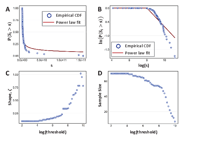
Figure 1 presents the revenue results graphically. Panel A and Panel B show the empirical CDF and Power Law fits in linear and logarithmic spaces, respectively, when total revenue is used as the firm size proxy. The Power law fit is found to be slightly heavier tailed than the empirical CDF.
Panel C plots the effect of threshold selection on the shape parameter estimates for firm size. We find that the estimates are sensitive to the threshold with higher values of threshold associated with higher values of . The threshold we select, $100,000,000 (, i.e. ), corresponds to a plateau, after which the shape parameter estimates are not stable.
It is also important to note that higher threshold values significantly decrease the sample size, which is plotted in Panel D of Figure 1. The effect of the sample size on the firm size distribution is tested by Segarra and Teruel (2012) using Spanish manufacturing firms for the years 2001 and 2006. Their findings indicate that the sample size inversely affects the estimated coefficient of firm size distribution. They find that estimates of tend to be larger () with small samples of large firms than compared to large samples that include smaller firms. The same finding applies for both sales and employees as the firm size proxy. In particular, in 2006, they find that the estimated of the largest 100 firms is 1.36 for sales and 1.66 for employees, respectively. However, when the whole sample of 60,000+ firms are considered, the parameter estimates decrease to 0.68 for sales and 0.97 for employees. They argue that increasing sample size has a negative effect on the power law parameter.
Table 5 shows the estimates of the production function given in Equation (12), using firm-level data from the U.S. Motor Vehicles and Parts sector. As discussed earlier, OLS and Fixed Effect estimates do not control for biases caused by simultaneity, and so we also consider OP and GMM estimates of the production function. We see that the OLS estimates for labor (capital) elasticity are slightly higher (lower) than the OP estimates. This is to be expected as coefficients associated with variable inputs (e.g., labor and materials) are expected to have an upward bias, and the coefficients associated with quasifixed inputs (e.g., capital) are expected to be biased downward (Olley and Pakes, 1996). Further, the Fixed Effect coefficient for capital elasticity is unreasonably low, which has been a known source of concern in the productivity literature Ackerberg et al. (2007).
| Method: | N | SE | SE | ||||
| OLS | 246 | 0.83*** | 0.05 | 0.25*** | 0.05 | ||
| Fixed Effects | 246 | 0.47* | 0.27 | 0.003 | 0.02 | ||
| Olley-Pakes | 189 | 0.80*** | 0.05 | 0.30*** | 0.03 | ||
| GMM | 189 | 0.70*** | 0.07 | 0.20 | 0.15 | ||
Firm-level studies generally show that there is a large and persistent difference in productivity between firms even within narrowly defined industries. Using all of our measures of productivity, we find that dispersion in the U.S. Motor Vehicles and Parts sector ranges from a low of 1.35 (OLS) to a high of 1.93 (LP), where dispersion is calculated as the difference between the 90th and the 10th percentile of log TFP. For the four-digit U.S. manufacturing industries, Syverson (2004) found a mean dispersion in the range of , and so the calculated dispersion in this sector is at the high end of these estimates. Our results thus suggest that there is more room for aggregate productivity increase in the U.S. Motor Vehicles and Parts sector as resources get reallocated from the less to the more productive firms.
Finally, we examine how the different productivity measures relate to one another. Table 6 shows the correlation between all of our calculated productivity measures. The correlations between labor productivity and the TFP estimates are generally high, around to . Similarly, correlations between the index-based TFP measure and the estimated TFP are also high, ranging from to . One exception is the TFP measure estimated with Fixed Effects which has a very low correlation of 22 percent with the index-based TFP measures. Turning to the relationship among estimated TFP measures, correlations are very high, reaching nearly one between OP and GMM estimates.18 Again though, the Fixed Effects based TFP measure shows low correlation with the other estimated TFP measures. Thus, given the earlier concerns over Fixed Effects estates, we only consider the OLS and OP methods for our estimation-based TFP measure in the subsequent analysis.
| LP | Solow | OLS | FE | OP | GMM | |
| LP | 1.00 | |||||
| Solow | 0.41 | 1.00 | ||||
| OLS | 0.80 | 0.75 | 1.00 | |||
| FE | 0.71 | 0.22 | 0.46 | 1.00 | ||
| OP | 0.72 | 0.74 | 0.97 | 0.38 | 1.00 | |
| GMM | 0.60 | 0.84 | 0.91 | 0.30 | 0.95 | 1.00 |
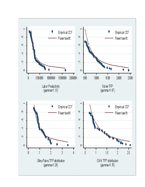
We next estimate the power law for our four chosen firm productivity measures: LP, Solow, OLS and OP. Table 7 shows the estimates of the shape parameter for each measure (Figure 2 shows the fit for each measure based on the MLE method). We see that there is some heterogeneity in these shape parameters based on the particular productivity measure as well as the estimation method used to identify the shape parameter. Despite these differences, the range of values takes is around , a relatively narrow interval. This increases our confidence that the shape parameter for the U.S. Motor Vehicles and Parts sector is relatively robust to various productivity and estimation methods. These estimates are also in line with Spearot (2016) which show a shape parameter, averaged across countries, of for the Motor Vehicles and Parts sector.
A small shape parameter around implies a large dispersion of productivity among firms, with low-productivity firms capturing a small share of the market. On the other hand, in an industry with a large shape parameter, there is a large mass of low-productivity firms that represent a larger share of industry output. di Giovanni and Levchenko (2013) show that in the case when the firm size distribution is fat-tailed (small shape parameter), the incumbent firms in the industry are large and have a disproportionate share of overall sales compared to the small marginal firms and the welfare impact of trade is driven by incumbent firms rather than the marginal ones. Therefore, the contribution of the extensive margin to trade in the U.S. Motor Vehicles and Parts sector will be relatively small from reductions in trade costs.
| Method: | (cdf) | (rank) | (mle) |
| LP | -1.72*** | 0.86*** | 1.11*** |
| (0.07) | (0.04) | (0.15) | |
| Solow | -2.40*** | 0.88*** | 1.67*** |
| (0.11) | (0.04) | (0.25) | |
| OP | -2.00*** | 1.67*** | 1.28*** |
| (0.12) | (0.09) | (0.18) | |
| GMM | -2.26*** | 1.70*** | 1.79*** |
| (0.13) | (0.09) | (0.27) | |
It is important to use appropriate values for the parameters in policy analysis because welfare predictions are highly sensitive to the value of the firm heterogeneity parameters. For instance, the elasticity of substitution translates the price differences across firms into differences in market shares and will have opposite effects on each margin of trade (Kancs, 2010; Hillberry and Hummels, 2013). As Kancs (2010) states, “the elasticity of substitution magnifies the sensitivity of the intensive margin to changes in trade barriers, whereas it dampens the sensitivity of the extensive margin” (Kancs, 2010, pp. 276). When the elasticity of substitution is high, the intensive margin is more sensitive to changes in trade barriers while the extensive margin is less sensitive. When elasticity is high, low-productivity firms are at a severe disadvantage because they can only capture a small market share. Therefore, their impact on trade flows is marginal and small. However, with a low substitution elasticity, each firm has more market power over their unique variety and are in a sense more sheltered from the productivity competition. Therefore, new entrants are able to capture a higher market share and make a larger impact on trade flows as well as welfare. Overall, the export sales by new entrants are largest when there is supply-side homogeneity (high ) and demand-side heterogeneity (low ) (Hillberry and Hummels, 2013).
The empirical work in previous sections allow us to find the shape parameter of firm size, , and the shape parameter of productivity distribution, . We use four different empirical methods to estimate TFP and three different methods to fit the TFP estimates to Pareto distribution. This exercise results in , possible estimates. We use two proxies for firm size and three methods to fit firm size to a Pareto distribution, and this results in possible estimates. When we use the and estimates to impute , we find possible values for the U.S. motor vehicles and parts sector. These values are provided in Table 8 .
As Table 8 shows, the estimators deliver slightly different results. When revenue is used as the firm size proxy, the average value of is found as 4.53. Overall, MLE method delivers higher values compared to CDF and ln(Rank-0.5). The highest value of 6.06 is obtained when productivity is estimated using GMM and firm size distribution fit is obtained by MLE. Estimates for are slightly lower when the number of employees is used as the firm size proxy. The average value in this case is 3.78. values across estimation methods vary slightly compared to the revenue columns.
| Method: | CDF | ln(Rank-0.5) | MLE |
| GMM | 4.90 | 4.40 | 6.42 |
| LP | 3.97 | 2.72 | 4.36 |
| OP | 4.45 | 4.34 | 4.88 |
| Solow | 5.14 | 2.76 | 6.06 |
All the
values found in Table 8 are high compared to the corresponding
values. Most importantly, they do not satisfy the mathematical constraint of
, which results from the
firm shape parameter of ,
as discussed in Section 5.1. As a counterfactual calibration analysis, we compare the
values in Table 8 to the benchmark Zipf’s Law where
, which
implies that .
Moreover, we compare them to the case where the mathematical constraint
is satisfied,
such as when .
The resulting parameter values are reported in Table 9 and 10.
| Method: | CDF | ln(Rank-0.5) | MLE |
| GMM | 3.26 | 2.70 | 2.79 |
| LP | 2.72 | 1.86 | 2.11 |
| OP | 3.00 | 2.67 | 2.28 |
| Solow | 3.40 | 1.88 | 2.67 |
| Method: | CDF | ln(Rank-0.5) | MLE |
| GMM | 2.13 | 1.85 | 1.90 |
| LP | 1.86 | 1.43 | 1.56 |
| OP | 2.00 | 1.84 | 1.64 |
| Solow | 2.20 | 1.44 | 1.84 |
The counterfactual analysis of delivers lower values for and deliver even lower values. Since the estimates for are small for U.S. Motor Vehicles and Parts, the corresponding values should also be accordingly small. Sectors characterized with high productivity heterogeneity tend to have differentiated varieties.
A growing literature incorporating firm heterogeneity in trade models has generated new economic insights on the overall impact of globalization. In the meantime, there still remain a number of empirical challenges for extending this broad framework to applied policy work. Model simulations have been shown to be quite sensitive to parameter values, thus making it paramount that the structural parameters are identified in a manner consistent with underlying theory, rather than relying on ad hoc values from other strands in the trade literature.
This paper addresses this gap in the literature by proposing a simple method to estimate the structural parameters of trade models with firm heterogeneity. When firm productivity follows a Pareto distribution with the shape parameter , firm size also follows Pareto distribution with shape parameter . We can thus estimate both distributions using the established approaches in the literature and then use the estimated and values to impute the corresponding values. Using the same database and distribution, our proposed method is able to consolidate the estimation of structural parameters within the firm heterogenity framework, thus ensuring better informed parameter values and more reliable model predictions.
We illustrate this methodology by focusing on the U.S. Motor Vehicles and Parts sector using the ORBIS database. The estimates for are found to be in line with the estimates in the literature for motor vehicles sector. However, they are slightly lower than the values found in the literature when all manufacturing firms are pooled. Similarly, the estimates for are in line with the literature for the motor vehicles sector. While the resulting values for are close to the elasticity estimates for manufacturing sectors, they do not satisfy the mathematical constraint for a well-defined firm heterogeneity model. We find that smaller values are required to satisfy the constraint given the estimates for .
A possible remedy to this finding could be to increase the sample size in the database. The number of observations for the U.S. Motor Vehicles Sector in our sample is relatively small which is found to result in smaller shape parameters for firm size distribution. Extending this analysis with a larger sample size is a potential venue for the next step of this study.
| Year | Observations | Mean | Std. Dev. | Min. | Max. | Median |
| 2008 | 2 | 140 | 198 | 0 | 280 | 140 |
| 2009 | 7 | 2,692 | 6,631 | 3 | 17,710 | 18 |
| 2010 | 23 | 2,150 | 8,684 | 0 | 41,946 | 221 |
| 2011 | 64 | 8,107 | 25,913 | 0 | 150,000 | 797 |
| 2012 | 64 | 8,299 | 26,294 | 0 | 152,000 | 866 |
| 2013 | 65 | 8,584 | 27,597 | 0 | 155,000 | 984 |
| 2014 | 65 | 8,920 | 27,884 | 0 | 156,000 | 980 |
| 2015 | 57 | 8,707 | 28,061 | 0 | 152,000 | 1,403 |
| 2016 | 39 | 12,910 | 35,158 | 3 | 166,000 | 2,810 |
| Year | Observations | Mean | Std. Dev. | Min. | Max. | Median |
| 2008 | 2 | 823 | 1,147 | 12 | 1,634 | 823 |
| 2009 | 6 | 8,173 | 19,189 | 16 | 47,326 | 94 |
| 2010 | 20 | 4,330 | 11,352 | 8 | 51,623 | 1,121 |
| 2011 | 61 | 17,537 | 38,683 | 2 | 207,000 | 3,319 |
| 2012 | 59 | 18,209 | 40,503 | 3 | 213,000 | 4,400 |
| 2013 | 54 | 20,518 | 43,596 | 2 | 219,000 | 5,327 |
| 2014 | 56 | 21,650 | 43,690 | 3 | 216,000 | 5,930 |
| 2015 | 49 | 23,747 | 47,068 | 12 | 215,000 | 6,700 |
| 2016 | 34 | 33,159 | 56,679 | 1,700 | 225,000 | 11,493 |
| Year | Observations | Mean | Std. Dev. | Min. | Max. | Median |
| 2008 | 2 | 41 | 57 | 0 | 81 | 41 |
| 2009 | 7 | 2,395 | 6,236 | 0 | 16,536 | 8 |
| 2010 | 22 | 765 | 3,260 | 0 | 15,352 | 39 |
| 2011 | 60 | 1,495 | 4,567 | 0 | 23,790 | 126 |
| 2012 | 63 | 1,556 | 4,891 | 0 | 25,845 | 142 |
| 2013 | 65 | 1,659 | 5,350 | 0 | 29,250 | 142 |
| 2014 | 64 | 1,826 | 6,060 | 0 | 34,803 | 153 |
| 2015 | 57 | 2,085 | 7,816 | 0 | 51,401 | 185 |
| 2016 | 39 | 3,866 | 12,379 | 0 | 70,346 | 366 |
| Year | Observations | Mean | Std. Dev. | Min. | Max. | Median |
| 2009 | 2 | 7 | 10 | 0 | 14 | 7 |
| 2010 | 7 | 252 | 653 | 0 | 1,733 | 1 |
| 2011 | 21 | 136 | 558 | -4 | 2,568 | 4 |
| 2012 | 61 | 397 | 1,350 | -22 | 8,057 | 24 |
| 2013 | 63 | 445 | 1,538 | -12 | 9,178 | 35 |
| 2014 | 63 | 499 | 1,992 | -783 | 12,115 | 26 |
| 2015 | 56 | 735 | 3,402 | -190 | 24,288 | 31 |
| 2016 | 39 | 1,509 | 5,210 | 0 | 29,025 | 85 |
Ackerberg, D., C. L. Benkard, S. Berry, and A. Pakes (2007). Econometric tools for analyzing market outcomes. Handbook of Econometrics 6, 4171–4276.
Akgul, Z., N. B. Villoria, and T. W. Hertel (2015). Theoretically-consistent parameterization of a multi-sector global model with heterogeneous firms. In 18th Annual Conference on Global Economic Analysis, Number 4731. 18th Annual Conference on Global Economic Analysis.
Akgul, Z., N. B. Villoria, and T. W. Hertel (2016, June). GTAP - HET: Introducing firm heterogeneity into the GTAP model. Journal of Global Economic Analysis 1(1), 111–180.
Anderson, J. E. and E. van Wincoop (2003). Gravity with gravitas: A solution to the border puzzle. American Economic Review 93(1), 170–192.
Arkolakis, C., S. Demidova, P. J. Klenow, and A. Rodriguez-Clare (2008, MAY). Endogenous variety and the gains from trade. American Economic Review 98(2), 444–450. 120th Annual Meeting of the American-Economic-Association, New Orleans, LA, JAN 04-06, 2008.
Axtell, R. L. (2001). Zipf distribution of US firm sizes. Science 293(5536), 1818–1820.
Balistreri, E. J., R. H. Hillberry, and T. F. Rutherford (2011). Structural estimation and solution of international trade models with heterogeneous firms. Journal of International Economics 83(2), 95–108.
Balistreri, E. J. and T. F. Rutherford (2013). Computing general equilibrium theories of monopolistic competition and heterogeneous firms. In P. B. Dixon and D. W. Jorgenson (Eds.), Handbook of Computable General Equilibrium Modeling.
Bernard, A. B., J. Eaton, J. B. Jensen, and S. Kortum (2003). Plants and productivity in international trade. American Economic Review 93(4), 1268–1290.
Bernard, A. B., J. B. Jensen, S. J. Redding, and P. K. Schott (2007). Firms in international trade. The Journal of Economic Perspectives 21(3), 105–130.
Bottazzi, G., D. Pirino, and F. Tamagni (2015, JUL). Zipf law and the firm size distribution: a critical discussion of popular estimators. Journal of Evolutionary Economics 25(3), 585–610.
Broda, C. and D. E. Weinstein (2006). Globalization and the gains from variety. Quarterly Journal of Economics 121(2), 541–585.
Chaney, T. (2008). Distorted gravity: The intensive and extensive margins of international trade. American Economic Review 98(4), 1707–1721.
Clauset, A., C. R. Shalizi, and M. E. Newman (2009). Power-law distributions in empirical data. SIAM review 51(4), 661–703.
Crozet, M. and P. Koenig (2010). Structural gravity equations with intensive and extensive margins. Canadian Journal of Economics-Revue Canadienne D Economique 43(1), 41–62.
Del Gatto, M., A. Di Liberto, and C. Petraglia (2011). Measuring productivity. Journal of Economic Surveys 25(5), 952–1008.
di Giovanni, J. and A. A. Levchenko (2013). Firm entry, trade, and welfare in zipf’s world. Journal of International Economics 89(2), 283–296.
di Giovanni, J., A. A. Levchenko, and R. Rancière (2011). Power laws in firm size and openness to trade: Measurement and implications. Journal of International Economics 85(1), 42–52.
Dixon, P. B., M. Jerie, and M. T. Rimmer (2016, June). Modern trade theory for CGE modelling: The Armington, Krugman and Melitz models. Journal of Global Economic Analysis 1(1), 1–110.
Eaton, J. and S. Kortum (2002). Technology, geography, and trade. Econometrica 70(5), 1741–1779.
Eaton, J., S. Kortum, and F. Kramarz (2011). An anatomy of international trade: Evidence from french firms. Econometrica 79(5), 1453–1498.
Feenstra, R. C. (2014, January). Restoring the product variety and pro-competitive gains from trade with heterogeneous firms and bounded productivity. National Bureau of Economic Research (19833).
Gabaix, X. (2009). Power Laws in Economics and Finance. Annual Review of Economics 1, 255–293.
Gabaix, X. and R. Ibragimov (2011, JAN). Rank-1/2: A Simple Way to Improve the OLS Estimation of Tail Exponents. Journal of Business & Economic Statistics 29(1), 24–39.
Gabaix, X. and Y. Ioannides (2004). Handbook of Regional and Urban Economics, Volume 4, Chapter The Evolution of City Sizes, pp. 2341–2378. North Holland, Amsterdam.
Gal, P. N. (2013). Measuring total factor productivity at the firm level using oecd-orbis. OECD Working Paper No. 1049.
Greenaway, D. and R. Kneller (2007). Firm heterogeneity, exporting and foreign direct investment. The Economic Journal 117(517), F134–F161.
Hayakawa, K., T. Machikita, and F. Kimura (2012). Globalization and productivity: A survey of firm-level analysis. Journal of Economic Surveys 26(2), 332–350.
Head, K. and T. Mayer (2014). Gravity equations: Workhorse,toolkit, and cookbook. In E. H. Gopinath, G and K. Rogoff (Eds.), Handbook of International Economics, Volume 4, Journal article 3, pp. 131–195. Elsevier.
Hertel, T., D. Hummels, M. Ivanic, and R. Keeney (2007). How confident can we be of cge-based assessments of free trade agreements? Economic Modelling 24(4), 611–635.
Hillberry, R. and D. Hummels (2013). Trade elasticity parameters for a computable general equilibrium model. In B. D. Peter and W. J. Dale (Eds.), Handbook of Computable General Equilibrium Modeling, Volume 1, Book section 18, pp. 1213–1269. Elsevier.
Kancs, D. (2010). Structural estimation of variety gains from trade integration in asia. Australian Economic Review 43(3), 270–288.
López, R. A. (2005). Trade and growth: Reconciling the macroeconomic and microeconomic evidence. Journal of Economic Surveys 19(4), 623–648.
McDaniel, C. and E. J. Balistreri (2003). A review of armington trade substitution elasticities. Integration and Trade 18(7), 161–173.
Melitz, M. J. (2003). The impact of trade on intra-industry reallocations and aggregate industry productivity. Econometrica 71(6), 1695–1725.
Melitz, M. J. and S. J. Redding (2013). Firm heterogeneity and aggregate welfare. National Bureau of Economic Research (18919).
Olley, G. S. and A. Pakes (1996). The dynamics of productivity in the telecommunications equipment industry. Econometrica 64(6), 1263–1297.
Petrin, A. K. and J. A. Levinsohn (2003). Estimating production functions using inputs to control for unobservables. Review of Economic Studies 70(2), 317–341.
Segarra, A. and M. Teruel (2012, APR). An appraisal of firm size distribution: Does sample size matter? Journal of Economic Behavior & Organization 82(1), 314–328.
Simonovska, I. and M. E. Waugh (2014, September). Trade models, trade elasticities, and the gains from trade. National Bureau of Economic Research (20495).
Solow, R. M. (1957). Technical change and the aggregate production function. The Review of Economics and Statistics, 312–320.
Spearot, A. (2016). Unpacking the long run effects of tariff shocks: New structural implications from firm heterogeneity models. AEJ Microeconomics 8(2), 128–67.
Syverson, C. (2004). Product substitutability and productivity dispersion. Review of Economics and Statistics 86(2), 534–550.
Van Beveren, I. (2012). Total factor productivity estimation: A practical review. Journal of Economic Surveys 26(1), 98–128.
Wagner, J. (2007). Exports and productivity: A survey of the evidence from firm-level data. The World Economy 30(1), 60–82.
Wooldridge, J. M. (2009). On estimating firm-level production functions using proxy variables to control for unobservables. Economics Letters 104(3), 112–114.
Yasar, M., R. Raciborski, B. Poi, et al. (2008). Production function estimation in stata using the olley and pakes method. Stata Journal 8(2), 221.
Zhai, F. (2008). Armington meets melitz: Introducing firm heterogeneity in a global CGE model of trade. Journal of Economic Integration 23(3), 575–604.
Zipf, G. (1950). Human behavior and the principle of least effort. Journal of Clinical Psychology 6(3), 306–306.
1There is an extensive literature on estimating trade elasticity using gravity models. See for example Anderson and van Wincoop (2003), Head and Mayer (2014) and Simonovska and Waugh (2014).
2For example, Spearot (2016) does not rely on a constant elasticity of substitution framework in estimating the shape parameters.
3Using French firm-level production data, di Giovanni et al. (2011) find close to 1 for their full sample of firms. However, when they separate the firms into exporting and non-exporting ones, the power law coefficient for exporters is consistently lower than the full sample of firms.
4In particular, when sales is used as the measure of firm size, they find to range around , depending on the particular estimation methodology. Results are similar when the number of employees is used as the measure of firm size.
5The LS estimation has generally been the more popular approach in the firm size distribution studies. However, in a test simulation, Clauset et al. (2009) show that the MLE has better performance, and that the LS regression methods can give significantly biased values. Thus we use both these approaches in our power law estimations.
6An extensive review by Bottazzi et al. (2015) discusses that neither CDF nor PDF log-log estimators have strong properties for unitary tail inference (Zipf’s Law) for firm size. They report that especially the PDF estimator performs very poorly with pooled data. They argue that and Maximum Likelihood estimators such as the Hill estimator prove to perform better, especially in small samples.
7See Hayakawa et al. (2012) for a broader survey on the causal mechanisms that allow productivity to have a key role in determining the effect trade has on the firm.
8See also López (2005), Greenaway and Kneller (2007) and Wagner (2007).
9As discussed in Wagner (2007), evidence regarding the learning-by-exporting is somewhat mixed with only few studies showing post-entry differences in productivity growth between exporters and non-exporters. So exporting, in itself, does not necessarily improve firm performance.
10To account for intermediate inputs, value added (revenue-cost of inputs) should be used as the measure of output. However, value added is not always available in a firm’s financial data. For example, many countries, including the U.S. do not require firms to provide information on material and labor costs, leading to insufficient coverage of value added measures in the ORBIS database.
11The labor share is averaged over the 2008-2015 period and does not vary in the subsequent calculations of the TFP.
12Ackerberg et al. (2007) note that if capital is positively correlated with labor and labor has a higher correlation with then will be upward biased while will be underestimated.
13See Van Beveren (2012) for a more detailed discussion.
14Petrin and Levinsohn (2003) extend this framework, by using inputs, such as electricity or materials, instead of investment to control for the firm’s unobserved productivity. These inputs usually have more non-zero observations than investment, and so increases the efficiency of TFP estimates when used with manufacturing surveys of developing countries. However, the financial data on the U.S. motor sector in ORBIS does not include a separate account for material costs, and so we continue to follow the OP framework in our analysis.
15To account for selection effects, OP also include a term for predicted probabilities in (16) where are obtained from a probit model on firm survival with and as the main explanatory variables. However, Levinson and Petrin (2003) show that incorporating survival probability only leads to very small efficiency gains and so we do not include a correction for selection bias in our analysis.
16We pool the year-firm observations for those firms that have not yet reported for 2016.
17Gal (2013) suggests using external sources to impute a firm’s missing labor costs. Relying on industry level data such as the OECD STAN database, average labor cost per worker in a particular sector can be obtained by dividing the total labor cost by the number of employees per country, year and 2-digit industry level. This average cost is then multiplied by the number of firm employees in ORBIS to get the imputed firm-specific labor costs. However, this approach will only work if within-industry wage differentials are not too prominent, a feature unlikely to hold in the U.S. where empirical evidence has generally shown productive firms paying a greater premium on wages.
18Gal (2012) also shows that in practice there was not a lot of difference when using these two TFP measures.